Combining CNN and RNN for spoken language identification
By Hrayr Harutyunyan and Hrant Khachatrian
Last year Hrayr used convolutional networks to identify spoken language from short audio recordings for a TopCoder contest and got 95% accuracy. After the end of the contest we decided to try recurrent neural networks and their combinations with CNNs on the same task. The best combination allowed to reach 99.24% and an ensemble of 33 models reached 99.67%. This work became Hrayr’s bachelor’s thesis.
Contents
Inputs and outputs
As before, the inputs of the networks are spectrograms of speech recordings. It seems spectrograms are the standard way to represent audio for deep learning systems (see “Listen, Attend and Spell” and “Deep Speech 2: End-to-End Speech Recognition in English and Mandarin”).
Some networks use up to 11khz frequencies (858 x 256 image) and others use up to 5.5khz frequencies (858 x 128 image). In general the networks which use up to 5.5khz frequencies perform a little bit better (probably because the higher frequencies do not contain much useful information and just make overfitting easier).
The output layer of all networks is a fully connected softmax layer with 176 units.
We didn’t augment the data using vocal tract length augmentation.
Network architecture
We have tested several network architectures. First set of architectures are plain AlexNet-like convolutional networks. The second set contains no convolutions and interprets the columns of the spectrogram as a sequence of inputs to a recurrent network. The third set applies RNN on top of the features extracted by a convolutional network. All models are implemented in Theano and Lasagne.
Almost all networks easily reach 100% accuracy on the training set. In the following tables we describe all architectures we tried and report accuracy on the validation set.
Convolutional networks (CNN)
The network consists of 6 blocks of 2D convolution, ReLU nonlinearity, 2D max pooling and batch normalization. We use 7x7 filters for the first convoluational layer, 5x5 for the second and 3x3 for the rest. Pooling size is always 3x3 with a stride 2.
Batch normalization significantly increases the training speed (this fact is reported in lots of recent papers). Finally we use only 1 fully connected layer between the last pooling layer and the softmax layer, and apply 50% dropout on that.
| Network | Accuracy | Notes |
|---|---|---|
| tc_net | <80% | The difference between this network and the CNN descibed in the previous work is that this network has only one fully connected layer. We didn’t train this network much because of ignore_border=False, which slows down the training |
| tc_net_mod | 97.14 | This network is the same as tc_net but instead of ignore_border=False, we put pad=2 |
| tc_net_mod_5khz_small | 96.49 | This network is a smaller copy of tc_net_mod network and works with up to 5.5khz frequencies |
The Lasagne setting ignore_border=False prevents Theano from using CuDNN. Setting it to True significantly increased the speed.
Here is the detailed description of the best network of this set: tc_net_mod.
| Nr | Type | Channels | Width | Height | Kernel size / stride |
|---|---|---|---|---|---|
| 0 | Input | 1 | 858 | 256 | |
| 1 | Conv | 16 | 852 | 250 | 7x7 / 1 |
| ReLU | 16 | 852 | 250 | ||
| MaxPool | 16 | 427 | 126 | 3x3 / 2, pad=2 | |
| BatchNorm | 16 | 427 | 126 | ||
| 2 | Conv | 32 | 423 | 122 | 5x5 / 1 |
| ReLU | 32 | 423 | 122 | ||
| MaxPool | 32 | 213 | 62 | 3x3 / 2, pad=2 | |
| BatchNorm | 32 | 213 | 62 | ||
| 3 | Conv | 64 | 211 | 60 | 3x3 / 1 |
| ReLU | 64 | 211 | 60 | ||
| MaxPool | 64 | 107 | 31 | 3x3 / 2, pad=2 | |
| BatchNorm | 64 | 107 | 31 | ||
| 4 | Conv | 128 | 105 | 29 | 3x3 / 1 |
| ReLU | 128 | 105 | 29 | ||
| MaxPool | 128 | 54 | 16 | 3x3 / 2, pad=2 | |
| BatchNorm | 128 | 54 | 16 | ||
| 5 | Conv | 128 | 52 | 14 | 3x3 / 1 |
| ReLU | 128 | 52 | 14 | ||
| MaxPool | 128 | 27 | 8 | 3x3 / 2, pad=2 | |
| BatchNorm | 128 | 27 | 8 | ||
| 6 | Conv | 256 | 25 | 6 | 3x3 / 1 |
| ReLU | 256 | 25 | 6 | ||
| MaxPool | 256 | 14 | 3 | 3x3 / 2, pad=2 | |
| BatchNorm | 256 | 14 | 3 | ||
| 7 | Fully connected | 1024 | |||
| ReLU | 1024 | ||||
| BatchNorm | 1024 | ||||
| Dropout | 1024 | ||||
| 8 | Fully connected | 176 | |||
| Softmax Loss | 176 |
During the training we accidentally discovered a bug in Theano, which was quickly fixed by Theano developers.
Recurrent neural networks (RNN)
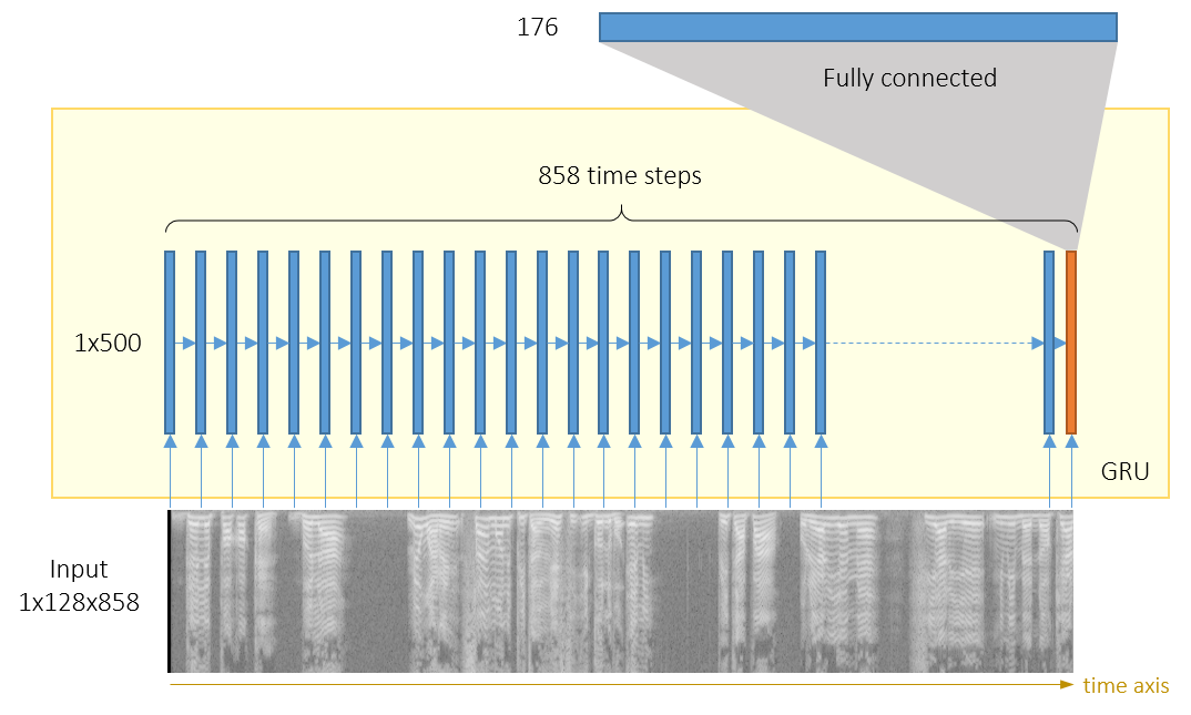
The spectrogram can be viewed as a sequence of column vectors that consist of 256 (or 128, if only <5.5KHz frequencies are used) numbers. We apply recurrent networks with 500 GRU cells in each layer on these sequences.

| Network | Accuracy | Notes |
|---|---|---|
| rnn | 93.27 | One GRU layer on top ot the input layer |
| rnn_2layers | 95.66 | Two GRU layers on top ot the input layer |
| rnn_2layers_5khz | 98.42 | Two GRU layers on top ot the input layer, maximum frequency: 5.5khz |
The second layer of GRU cells improved the performance. Cropping out frequencies above 5.5KHz helped fight overfitting. We didn’t use dropout for RNNs.
Both RNNs and CNNs were trained using adadelta for a few epochs, then by SGD with momentum (0.003 or 0.0003) until overfitting. If SGD with momentum is applied from the very beginning, the convergence is very slow. Adadelta converges faster but usually doesn’t reach high validation accuracy.
Combinations of CNN and RNN
The general architecture of these combinations is a convolutional feature extractor applied on the input, then some recurrent network on top of the CNN’s output, then an optional fully connected layer on RNN’s output and finally a softmax layer.
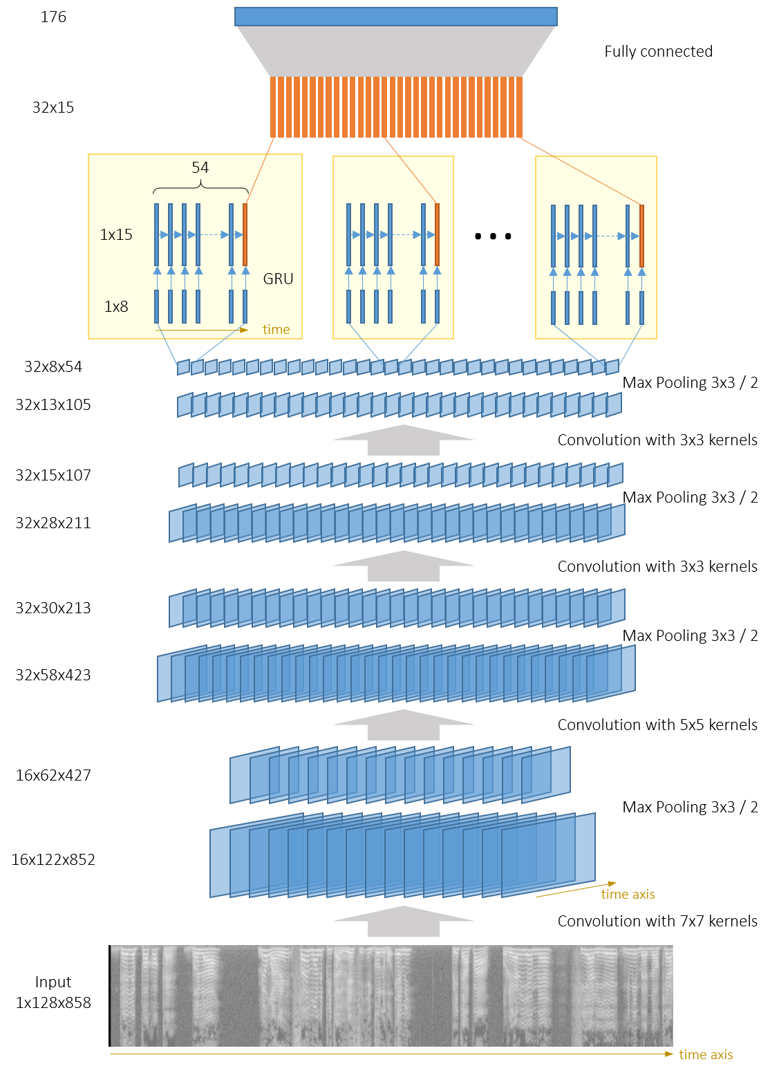
The output of the CNN is a set of several channels (also known as feature maps). We can have separate GRUs acting on each channel (with or without weight sharing) as described in this picture:

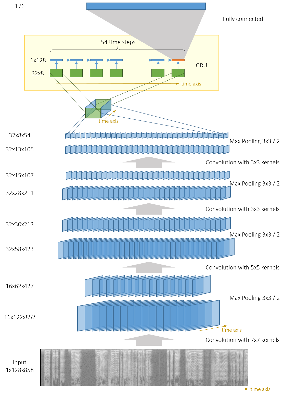
Another option is to interpret CNN’s output as a 3D-tensor and run a single GRU on 2D slices of that tensor:

The latter option has more parameters, but the information from different channels is mixed inside the GRU, and it seems to improve performance. This architecture is similar to the one described in this paper on speech recognition, except that they also use some residual connections (“shortcuts”) from input to RNN and from CNN to fully connected layers. It is interesting to note that recently it was shown that similar architectures work well for text classification.
| Network | Accuracy | Notes |
|---|---|---|
| tc_net_rnn | 92.4 | CNN consists of 3 convolutional blocks and outputs 32 channels of size 104x13. Each of these channels is fed to a separate GRU as a sequence of 104 vectors of size 13. The outputs of GRUs are combined and fed to a fully connected layer |
| tc_net_rnn_nodense | 91.94 | Same as above, except there is no fully connected layer on top of GRUs. Outputs of GRU are fed directly to the softmax layer |
| tc_net_rnn_shared | 96.96 | Same as above, but the 32 GRUs share weights. This helped to fight overfitting |
| tc_net_rnn_shared_pad | 98.11 | 4 convolutional blocks in CNN using pad=2 instead of ignore_broder=False (which enabled CuDNN and the training became much faster). The output of CNN is a set of 32 channels of size 54x8. 32 GRUs are applied (one for each channel) with shared weights and there is no fully connected layer |
| tc_net_deeprnn_shared_pad | 95.67 | 4 convolutional block as above, but 2-layer GRUs with shared weights are applied on CNN’s outputs. Overfitting became stronger because of this second layer |
| tc_net_shared_pad_augm | 98.68 | Same as tc_net_rnn_shared_pad, but the network randomly crops the input and takes 9s interval. The performance became a bit better due to this |
| tc_net_rnn_onernn | 99.2 | The outputs of a CNN with 4 convolutional blocks are grouped into a 32x54x8 3D-tensor and a single GRU runs on a sequence of 54 vectors of size 32*8 |
| tc_net_rnn_onernn_notimepool | 99.24 | Same as above, but the stride along the time axis is set to 1 in every pooling layer. Because of this the CNN outputs 32 channels of size 852x8 |
The second layer of GRU in this setup didn’t help due to the overfitting.
It seems that subsampling in the time dimension is not a good idea. The information that is lost during subsampling can be better used by the RNN. In the paper on text classification by Yijun Xiao and Kyunghyun Cho, the authors even suggest that maybe all pooling/subsampling layers can be replaced by recurrent layers. We didn’t experiment with this idea, but it looks very promising.
These networks were trained using SGD with momentum only. The learning rate was set to 0.003 for around 10 epochs, then it was manually decreased to 0.001 and then to 0.0003. On average, it took 35 epochs to train these networks.
Ensembling
The best single model had 99.24% accuracy on the validation set. We had 33 predictions by all these models (there were more than one predictions for some models, taken after different epochs) and we just summed up the predicted probabilities and got 99.67% accuracy. Surprisingly, our other attempts of ensembling (e.g. majority voting, ensemble only on some subset of all models) didn’t give better results.
Final remarks
The number of hyperparameters in these CNN+RNN mixtures is huge. Because of the limited hardware we covered only a very small fraction of possible configurations.
The organizers of the original contest did not publicly release the dataset. Nevertheless we release the full source code on GitHub. We couldn’t find many Theano/Lasagne implementations of CNN+RNN networks on GitHub, and we hope these scripts will partially fill that gap.
This work was part of Hrayr’s bachelor’s thesis, which is available on academia.edu (the text is in Armenian).