Diabetic retinopathy detection contest. What we did wrong
After watching the awesome video course by Hugo Larochelle on neural nets (more on this in the previous post) we decided to test our knowledge on some computer vision contest. We looked at Kaggle and the only active competition related to computer vision (except for the digit recognizer contest, for which lots of perfect out-of-the-box solutions exist) was the Diabetic retinopathy detection contest. This was probably quite hard to become our very first project, but nevertheless we decided to try. The team included Karen, Tigran, Hrayr, Narek (1st to 3rd year bachelor students) and me (PhD student). Long story short, we finished at the 82nd place out of 661 participants, and in this post I will describe in details what we did and what mistakes we made. All required files are on these 2 github repositories. We hope this will be interesting for those who just start to play with neural networks. Also we hope to get feedback from experts and other participants.
Contents
- The contest
- Software and hardware
- Image preprocessing
- Data augmentation
- Choosing training / validation sets
- Convolutional network architecture
- Loss function
- Preparing submissions
- Attempts to ensemble
- Acknowledgements
The contest
Diabetic retinopathy is a disease when the retina of the eye is damaged due to diabetes. It is one of the leading causes of blindness in the world. The contest’s aim was to see if computer programs can diagnose the disease automatically from the image of the retina. It seems the winners slightly surpassed the performance of general ophthalmologists.
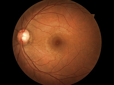
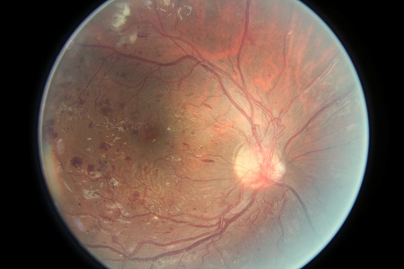
Each eye of the patient can be in one of the 5 levels: from 0 to 4, where 0 corresponds to the healthy state and 4 is the most severe state. Different eyes of the same person can be at different levels (although some contestants managed to leverage the fact that two eyes are not completely independent). Contestants were given 35126 JPEG images of retinas for training (32.5GB), 53576 images for testing (49.6GB) and a CSV file where level of the disease is written for the train images. The goal was to create another CSV file where disease levels are written for each of the test images. Contestants could submit maximum 5 CSV files per day for evaluation.
 |
 |
|---|---|
| Healthy eye: level 0 | Severe state: level 4 |
The score was evaluated using a metric called quadratic weighted kappa. It is described as being an agreement between two raters: the agreement between the scores assigned by human rater (which is unknown to contestants) and the predicted scores. If the agreement is random, the score is close 0 (sometimes it can even be negative). In case of a perfect agreement the score is 1. It is quadratic in a sense that, for example, if you predict level 4 for a healthy eye, it is 16 times worse than if you predict level 1. Winners achieved a score more than 0.84. Our best result was around 0.50.
Software and hardware
It was obvious that we were going to use a convolutional neural network for predicting. Not only because of its awesome performance on many computer vision problems, including another Kaggle competition on plankton classification, but also because it was the only technique we knew for image classification. We were aware of several libraries that implement convolutional networks, namely Python-based Theano, Caffe written in C++, cxxnet (developed by the 2nd place winners of the plankton contest) and Torch. We chose Caffe because it seemed to be the simplest one for beginners: it allows to define the neural network by a simple text file (like this) and train a network without writing a single line of code.
We didn’t have a computer with CUDA-enabled GPU in the university, but our friends at Cyclop Studio donated us an Intel Core i5 computer with 4GB RAM and NVidia GeForce GTX 550 TI card. 550 TI has a 1GB of memory which forced us to use very small batch sizes for the neural network. Later we switched to GeForce GTX 980 with 4GB memory, which was completely fine for us.
Karen and Tigran managed to install Caffe on Ubuntu and make it work with CUDA, which was enough to start the training. Later Narek and Hrayr found out how to play with Caffe models using Python, so we can run our models on the test set. Karen has connected Cloud9 to the server, and we could work remotely through a web interface.
Image preprocessing
Images from the training and test datasets have very different resolutions, aspect ratios, colors, are cropped in various ways, some are of very low quality, are out of focus etc. Neural networks require a fixed input size, so we had to resize / crop all of them to some fixed dimensions. Karen and Tigran looked at many sample images and decided that the optimal resolution which preserves the details required for classification is 512x512. We thought that in 256x256 we might lose the small details that differ healthy eye images from level 1 images. In fact, by the end of the competition we saw that our networks cannot differentiate between level 0 and 1 images even with 512x512, so probably we could safely work on 256x256 from the very beginning (which would be much faster to train). All preprocessing was done using imagemagick.
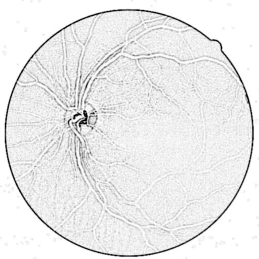
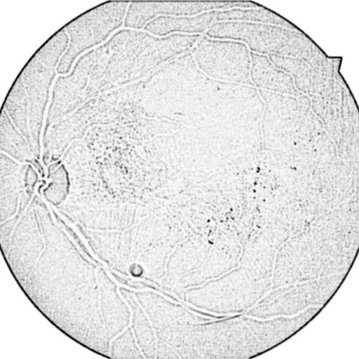
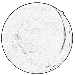
We tried three methods to preprocess the images. First, as suggested by Karen and Tigran, we resized the images and then applied the so called charcoal effect which is basically an edge detector. This highlighted the signs of blood on the retina. One of the challenging problems throughout the contest was to define a naming convention for everything: databases of preprocessed images, convnet descriptions, models, CSV files etc. We used the prefix edge for anything which was based on the images preprocessed this way. The best kappa score achieved on this dataset was 0.42.
 |
 |
|---|---|
| Preprocessed image (edge) level 0 | Preprocessed image (edge) level 3 |
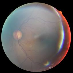
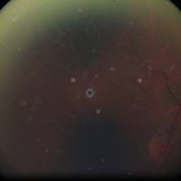
But later we noticed that this method makes the dirt on lens or other optical issues appear similar to a blood sign, and it really confused our neural networks. The following two images are of healthy eyes (level 0), but both were recognized by almost all our models as level 4.
 |
 |
|---|---|
 |
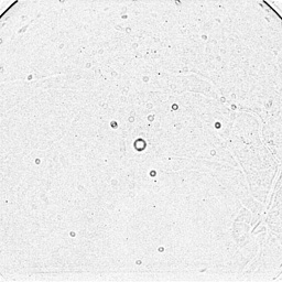 |
| Original images of healthy eyes | Preprocessed versions edge recognized as level 4 |
So we decided to avoid using filters on the images, and leave all the work to the convolutional network: just resize and convert to one channel image (to save space and memory). We thought that the color information is not very important to detect the disease, although this could be one of our mistakes. Following the discussion at Kaggle forums we decided to use the green channel only. We got our best results (kappa = 0.5) on this dataset. We used prefix g for these images.
Finally we tried to apply the equalize filter on top of the green channel, which makes the histogram of the image uniform. The best kappa score we managed to get on the dataset preprocessed this way was only 0.4. We used prefix ge for these images.
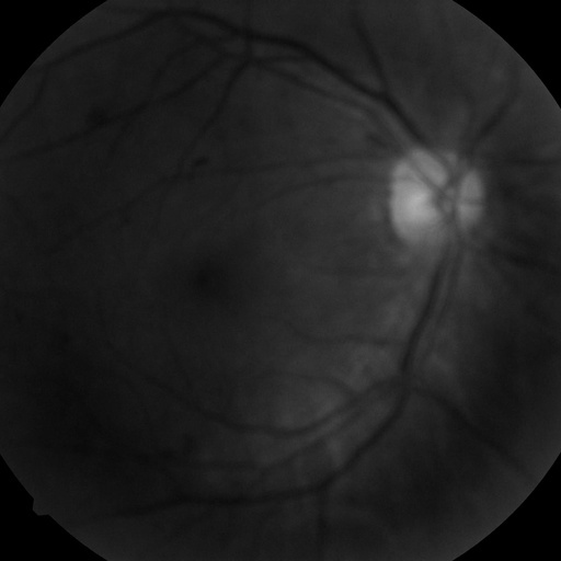 |
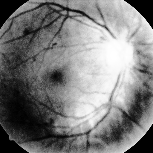 |
|---|---|
Just the green channel: g |
Histogram equalization on top of the green channel: ge |
Data augmentation
One of the problems of neural networks is that they are extremely powerful. They learn so well that they usually learn something that degrades their performance on other (previously unseen) data. One (made-up) example: the images in the training set are taken by different cameras and have different characteristics. If for some reason, say, the percentage of images of level 2 in dark images is higher than in general, the network may start to predict level 2 more often for dark images. We are not aware of any way to detect such “misleading” correlations by looking at neuron activations of convolution filters. But, fortunately, it is possible to train the network on one subset of data and test it on another, and if the performance on these subsets are different, then the network has learned something very specific to the training data, it has overfit the training data, and we should try to avoid it.
One of the solutions to this problem is to enlarge the dataset in order to minimize the chances of such correlations to happen. This is called data augmentation. The organizers of this contest explicitly forbid to use data outside the dataset they provided. But it’s obvious that if you take an image, zoom it, rotate it, flip it, change the brightness etc. the level of the disease will not be changed. So it is possible to apply these transformations to the images and obtain much larger and “more random” training dataset. One approach is to take all versions of all images into the training set, another approach is to randomly choose one transformation for each of the images. The mixture of these approaches helps to solve another problem which will be discussed in the next section.
We applied very limited transformations only. For every image we created 4 samples: original, rotated by 180 degrees, and the vertical flipped versions of these two. This helped to avoid the problem, that some of the images in the dataset were flipped.
We believe that we spent way too little time on data augmentation. All other contestants we have seen use much more sophisticated transformations. Probably this was our most important mistake.
Choosing training / validation sets
There are two reasons to train the networks only on a subset of the train dataset provided by Kaggle. First reason is to be able to compare different models. We need to choose the model which generalizes best to the unseen data, not the one which performs best on the data it has been trained on. So we train various models on some subset of the dataset (again called a training set), then compare their performance on the other subset (called a validation set) and pick the one which works better on the latter.
The second reason is to detect overfitting while training. During the training we sometimes (in Caffe this is configured by the test_interval parameter) run the network on the validation set and calculate the loss. When we see that the loss on the validation set does not decrease anymore, we know that overfitting happens. This is best illustrated in this image from Wikipedia.
The distribution of images of different levels in the training set provided by Kaggle was very uneven. More than half of the images were of healthy eyes:
| Level | Number of images | Percentage |
| 0 | 25810 | 73.48% |
| 1 | 2443 | 6.95% |
| 2 | 5292 | 15.07% |
| 3 | 873 | 2.49% |
| 4 | 708 | 2.02% |
Neural networks seem to be very sensitive to this kind of distributions. Our very first neural network (using softmax classification) was randomly giving labels 0 and 2 to almost all images (which brought a kappa score 0.138). So we had to make the classes more or less equal. Here we did couple of trivial mistakes.
At first we augmented the dataset by creating lots of rotations (multiples of 30 degrees, 12 versions of each image) and created a dataset of around 100K images with equally distributed classes. So we took 36 times more versions of images of level 4 than of images of level 0. As we had only 12 versions of each image, we took every image 3 times. Finally, we separated the training and validation sets after these augmentations. After training 88000 iterations (with batch size 2, we were still on GeForce 550 Ti) we had 0.55 kappa score on our validation set. But on Kaggle’s test set the score was only 0.23. So we had a terrible overfitting and didn’t detect it locally.
The most important point here, as I understand it, is that the separation of training and validation sets should have been done before the data augmentation. In our case we had different rotations of the same image in both sets, which didn’t allow us to detect overfitting.
So later we took 7472 images (21%) as a validation set, and performed the data augmentation on the remaining 27654 images. Validation set had the same ratio of classes as the Kaggle’s test set. This is important for choosing the best model: validation set should be similar to the test set as much as possible.
Also we decided to get rid off the rotations by multiples of 30 degrees, as the images were being distorted (we applied rotations after resizing the images). Although, after the competition we saw that other contestants have used such rotations. So maybe this was another mistake.
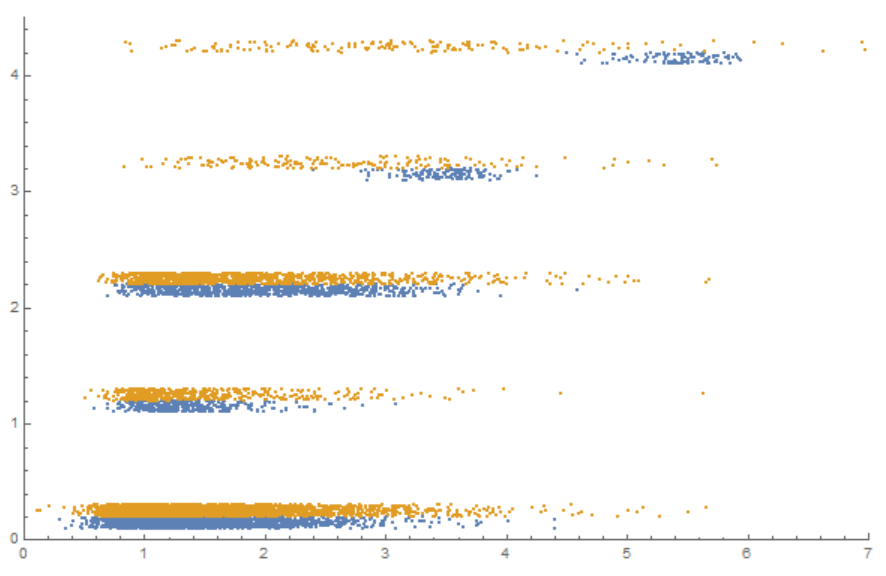
Then, it turned out that the idea of taking copies of the same image is terrible, because the network overfits the smaller classes (like level 3 and level 4) and it is hard to notice that just by looking at validation loss values, because the corresponding classes are very small in the validation set. We identified this problem by carefully visualizing neuron activations on training and validation sets (just 2 weeks before the competition deadline):
 |
|---|
Every dot corresponds to one image. Blue dots are from the training set, orange dots are from the validation set. x axis is the activation of a top layer neuron. y axis is the original label (0 to 4). Basically there is no overfitting for the images of level 0, 1 or 2: the activations are very similar. But the overfitting of the images of level 3 and 4 is obvious. Training samples are concentrated around fixed values, while validation samples are spread widely |
Finally we decided to train a network to differentiate between two classes only: images of level 0 and 1 versus images of level 2, 3 and 4. The ratio of the images in these classes was 4:1. We augmented the training set only by vertical flipping and rotating by 180 degrees. We took all 4 versions of each image of the second class and we randomly took one of the 4 versions of each image of the first class. This way we ended up with a training set of two equal classes. This gave us our best kappa score 0.50.
Later we wanted to train a classifier which would differentiate level 0 images from level 1 images only, but the networks we tried didn’t work at all. Another classifier we used to differentiate between level 2 and level 3 + level 4 images actually learned something, but we couldn’t increase the overall kappa score based on that.
After preparing the list of files for the training and validation sets, we used a tool bundled with Caffe to create a LevelDB database from the directory of images. Caffe prefers to read from LevelDB rather than from directory:
./build/tools/convert_imageset -backend=leveldb -gray=true -shuffle=true data/train.g/ train.g.01v234.txt leveldb/train.g.01v234gray is set to true because we use single-channel images and shuffle is required to properly shuffle the images before importing into the database.
Convolutional network architecture
Our best performing neural network architecture and corresponding solver are on Github. Batch size was always fixed to 20 (on GTX 980 card). We used a simple stochastic gradient descent with 0.9 momentum and didn’t touch learning rate policy at all (it didn’t decrease the rate significantly). We started at 0.001 learning rate, and sometimes manually decreased it (but not in this particular case which brought the best kappa score). Also in this best performing case we started with 0 weight decay, and after the first signs of overfitting (after 48K iterations, which is almost 20 epochs) increased it to 0.0015.
Convolution was done similar to the “traditional” LeNet architecture (developed by Yann LeCun, who invented the convolutional networks): one max pooling layer after every convolution layer, with fully connected layers at the end.
Almost all other contestants used the other famous approach, with multiple consecutive convolutional layers with small kernels before a pooling layer. This was developed by Karen Simonyan and Andrew Zisserman at Visual Geometry Group, University of Oxford (that’s why it is called VGGNet or OxfordNet) for the ImageNet 2014 contest where they took 1st and 2nd places for localization and classification tasks, respectively. Their approach was popularized by Andrej Karpathy and was successfully used in the plankton classification contest. I have tried this approach once, but it required significantly more memory and time, so I quickly abandoned it.
Here is the structure of our network:
| Nr | Type | Batches | Channels | Width | Height | Kernel size / stride |
| 0 | Input | 20 | 1 | 512 | 512 | |
| 1 | Conv | 20 | 40 | 506 | 506 | 7x7 / 1 |
| 2 | ReLU | 20 | 40 | 506 | 506 | |
| 3 | MaxPool | 20 | 40 | 253 | 253 | 3x3 / 2 |
| 4 | Conv | 20 | 40 | 249 | 249 | 5x5 / 1 |
| 5 | ReLU | 20 | 40 | 249 | 249 | |
| 6 | MaxPool | 20 | 40 | 124 | 124 | 3x3 / 2 |
| 7 | Conv | 20 | 40 | 120 | 120 | 5x5 / 1 |
| 8 | ReLU | 20 | 40 | 120 | 120 | |
| 9 | MaxPool | 20 | 40 | 60 | 60 | 3x3 / 2 |
| 10 | Conv | 20 | 40 | 56 | 56 | 5x5 / 1 |
| 11 | ReLU | 20 | 40 | 56 | 56 | |
| 12 | MaxPool | 20 | 40 | 14 | 14 | 4x4 / 4 |
| 13 | Fully connected | 20 | 256 | |||
| 14 | ReLU | 20 | 256 | |||
| 15 | Dropout | 20 | 256 | |||
| 16 | Fully connected | 20 | 256 | |||
| 17 | ReLU | 20 | 256 | |||
| 18 | Dropout | 20 | 256 | |||
| 19 | Fully connected | 20 | 1 | |||
| 20 | Euclidean Loss | 1 | 1 |
Some observations related to the network architecture:
- ReLU activations on all convolutional and fully connected layers helped a lot, kappa score increased by almost 0.1. It’s interesting to note that Christian Szegedy, one of the GoogLeNet developers (winner of the classification contest at ImageNet 2014), expressed an opinion that the main reason for the deep learning revolution happening now is the ReLU function :)
- 2 fully connected layers (256 neurons each) at the end is better than one fully connected layer. Kappa was increased by almost 0.03
- Number of filters in the convolutional layers are not very important. Difference between, say, 20 and 40 filters is very little
- Dropout helps fight overfitting (we used 50% probability everywhere)
- We didn’t notice any difference with Local response normalization layers
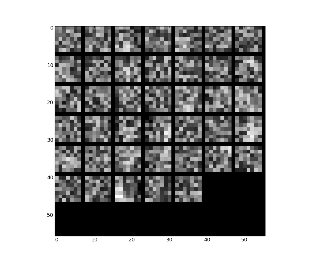
Below are the 40 filters of the first convolutional layer of our best model (visualization code is adapted from here). They don’t seem to be very meaningful:
I tried to use dropout on convolutional layers as well, but couldn’t make the network learn anything. The loss was quickly becoming nan. Probably the learning rate should have been very different…
Loss function
Submissions of this contest were evaluated by the metric called quadratic weighted kappa. We found an Excel code that implements it which helped us to get some intuition.
At the beginning we started to use softmax loss on top of the 5 neurons of the final fully connected layer. Later we decided to use something that will take into account the fact that the order of the labels matters (0 and 1 are closer than 0 and 4). We left only one neuron in the last layer and tried to use Euclidean loss. We even tried to “scale” the labels of the images in a way that will make it closer to being “quadratic”: we replaced the labels [0,1,2,3,4] with [0,2,3,4,6].
Ideally we would like to have a loss function that implements the kappa metric. But we didn’t risk to implement a new layer in Caffe. Jeffrey De Fauw has implemented some continuous approximation of kappa metric using Theano with a lot of success.
When we switched to 0,1 vs 2,3,4 classification, I thought 2-neuron softmax would be better than Euclidean loss because of the second neuron: it might bring some information that could help to obtain better score. But after some tests I saw that the sum of the activations of the two softmax neurons tends to 1, so the second neuron does not bring new information. The rest of the training was done using Euclidean loss (although I am not sure if that was the best option).
We logged the output of Caffe into a file, then plotted the graphs of training and validation losses using a Python script written by Hrayr:
./build/tools/caffe train -solver=solver.prototxt &> log_g_g_01v234_40r-2-40r-2-40r-2-40r-4-256rd0.5-256rd0.5-wd0-lr0.001.txt

python plot_loss.py log_g_01v234_40r-2-40r-2-40r-2-40r-4-256rd0.5-256rd0.5-wd0-lr0.001.txt
The script allows to print multiple logs on the same image and uses moving average to make the graph look smoother. It correctly aligns the graphs even if the log does not start from the first iteration (in case the training is resumed from a Caffe snapshot). For example, in the plot below train 1 and val 1 correspond to the model described in the previous section with weight decay=0; train 2 and val 2 correspond to the model which started from the 48000th iteration of the previous model but used weight decay=0.0015. The best kappa score was obtained on 81000th iteration of the second model. Then we observe overfitting.
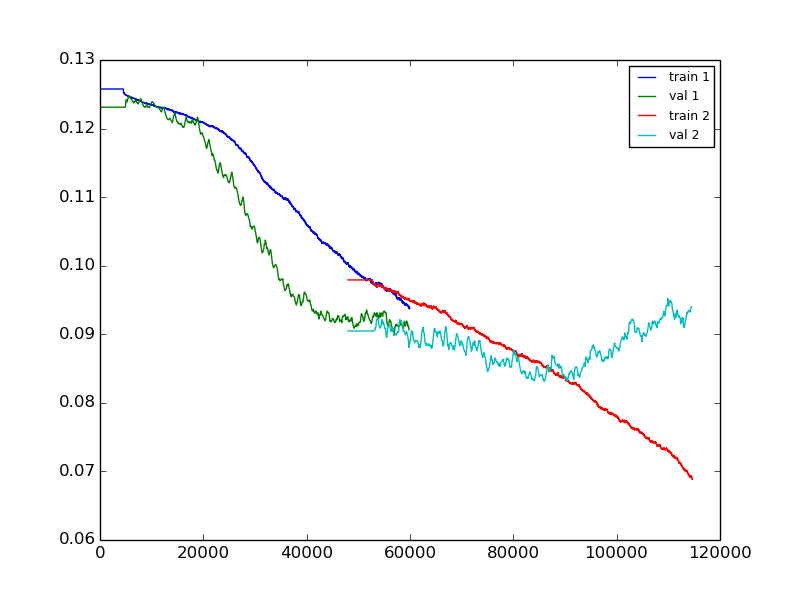
Note that the validation loss is usually lower than the training loss. The reason is that the classes are equal in the training set and are far from being equal in the validation set. So the training and validation losses cannot be compared.
Preparing submissions
After training the models we used a Python script to make predictions for the images in validation set. It creates a CSV file with neuron activations. Then we imported this CSV into Wolfram Mathematica and played with it there.
I use Mathematica mainly because of its nice visualizations. Here is one of them: the x axis is the activation of the single neuron of the last layer, and the graphs present the percentages of the images of each particular label that have x activation. Ideally the graphs corresponding to different labels should be clearly separable by vertical lines. Unfortunately that’s not the case, which visually explains why the kappa score is so low.
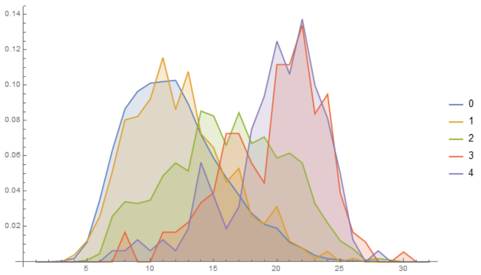
In order to convert the neuron activations to predicted levels we need to determine 4 “threshold” numbers. These graphs show that it’s not obvious how to choose these 4 numbers in order to maximize the kappa score. So we take, say, 1000 random 4-tuples of numbers between minimum and maximum activations of the neuron, and calculate the kappa score for each of the tuples. Then we take the 4-tuple for which the kappa was maximal, and use these numbers as thresholds for the images in the test set.
Note that we calculate the kappa scores for the validation set, although there is a risk to overfit the validation set. Ideally we should choose those thresholds which attain maximum kappa score on the train set. But, in practice, the thresholds that maximize the kappa score on validation set perform better on the test set, mainly because the network has already overfit the training set!
Attempts to ensemble
Usually it is possible to improve the scores by merging several models. This is called ensembling. For example, the 3rd place winners of this contest have merged the results of 9 convolutional networks.
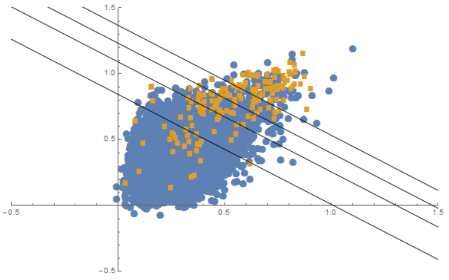
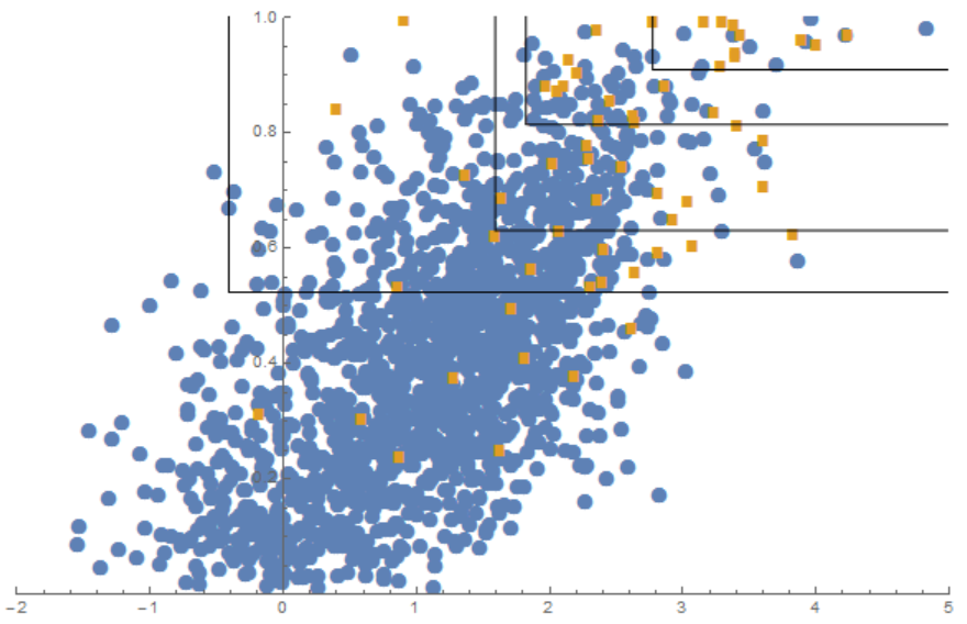
We developed couple of ways to merge the results from two networks, but they didn’t work well for us. They gave very small improvements (less than 0.01) only when both networks gave similar kappa scores. When one network was clearly stronger than the other one, the ensemble didn’t help at all. One of our ensemble methods was an extension of the “thresholding” method described in the previous section to 2 dimensions. We plot the images on a 2D plane in a way that each of the coordinates corresponds to a neuron activation of one model. Then we looked for random lines that split the plane in a way that maximizes the kappa score. We tried two methods of splitting the plane which are demonstrated below. Each blue dot corresponds to an image of label 0, orange dots correspond of images having label 4.
 |
 |
We didn’t try to merge more than 2 networks at once. Probably this was another mistake.
The only method of ensembling that worked for us was to take an average over 4 rotated / flipped versions of the images. We also tried to take minimum, maximum and harmonic mean of the neuron activations. Minimum and maximum brought 0.01 improvement to the kappa score, while harmonic and arithmetic means brought 0.02 improvement. The best result we achieved used the arithmetic mean. Note that this required to have 4 versions of test images (which took 2 days to rotate / flip) and to run the network on all versions (which took another day).
All these experiments can be replicated in Mathematica by using the script main.nb and the required CSV files that are available on Github.
Finally, note that Mathematica is the only non-free software used in the whole training process. We believe it is better to keep the ecosystem clean :) We will probably use IPython next time.
Many contestants have published their solutions. Here are the ones I could find. Please, let me know if I missed something. Most of the solution are heavily influenced by the winner method of the plankton classification contest.
- 1st place: Min-Pooling used OpenCV to preprocess the images, augmented the dataset by scaling, skewing and rotating (and notably not by changing colors), trained several networks on his own SparseConvNet library and used random forests to combine predictions from two eyes of the same person. Kappa = 0.84958
- 2nd place: o_O team used Theano, Lasagne, nolearn to train OxfordNet-like network on minimal preprocessed images. They have heavily augmented the dataset. They note the importance of using larger images to achieve high scores. Kappa = 0.84479
- 3rd place: Reformed Gamblers team combined results of 9 convolutional networks (OxfordNet-like and others) with leaky ReLU activations and non-trivial loss functions. They used Torch on multiple GPUs. Kappa = 0.83937
- Update: 4th place: Julian and Daniel gave an interview to Kaggle. They did extensive preprocessing and data augmentation, used CXXNet, PyLearn and Keras to train multiple OxfordNet-like networks. They highlight the importance of good parameter initialization.
- 5th place: Jeffrey De Fauw used Theano to train OxfordNet-like network with leaky ReLU activations on significantly augmented dataset. He has also implemented a smooth approximation of kappa metric and used it as a loss layer. Well written blog post. Kappa = 0.82899
- 20th place: Ilya Kavalerov, again Theano, OxfordNet, good augmentation, non-obvious loss function. Interesting read. Kappa = 0.76523
- 46th place: Niko Gamulin used Caffe on GTX 980 GPU (just like us) but OxfordNet architecture. Kappa = 0.63129
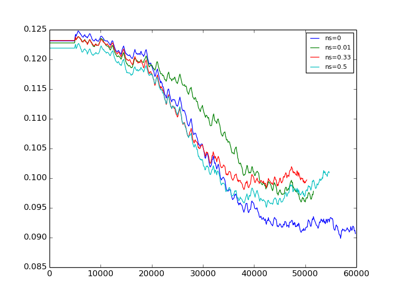
After the contest we tried to use leaky ReLUs, something we just didn’t think of during the contest. The results are not promising. Here are the plots of the validation losses with negative slope values (ns) 0, 0.01, 0.33 and 0.5 respectively:
Finally, Hrayr suggested to use different learning rates for different convolutional layers (Caffe supports this by specifying multiplication constants per layer). He used larger coefficients (12) for the first layers than for the top layers. The full prototxt file is on Github. This network allowed to get up to 0.52 kappa score on the local validation set. We didn’t try to run it on test images, although in almost all cases our scores on private leaderboard were higher than the scores on local validation sets.
Acknowledgements
We would like to express gratitude to Hugo Larochelle for his excellent video course on neural networks. After watching the videos we could easily understand almost all the terms in Caffe documentation.
We would like to thank the organizers of the contest for a great competition and the contestants for helpful discussions in forums and published solutions. We learned a lot from this contest.